Modelling the Agriculture Sector Value Added for the Kenyan Economy

Introduction

Brief Overview of the Kenyan Economy

Kenya continually followed an export-oriented agriculture-based growth policy, particularly in the early years of post-independence. During this period, agriculture was the backbone of the economy, implying that the economic performance of the country relied heavily on developments in the export market, weather conditions, and the government policy of the day. In the first fifteen years of independence, economic performance was impressive, with real GDP growing at an average 7 percent per annum while exports constituted 30 percent of the GDP. The fiscal deficit was largely contained.

The global shocks of the late 1970s and the drought experienced in the Horn of Africa in the early 1980s slowed down economic growth. This resulted in macroeconomic imbalances with double-digit inflation and a widened fiscal deficit.  In the wake of these developments, the government implemented structural adjustment programs (SAPs) between 1981 and 1989. SAPs consisted of a set of economic policies designed to generate rapid and sustainable economic growth with macroeconomic stability. These policies emphasized price decontrols, currency devaluation, and upward adjustment of smallholder producer prices, coming at a time when the main GDP contributor was agriculture.

Today, Kenya boasts of a youthful, skilled, and educated labor. The services industry is the main contributor to GDP (55%), followed by Agriculture, and thirdly, Manufacturing. In the 2000s, oil reserves were discovered in northern Kenya, with tests having been done on oil exploration in the country. Tapping into the oil and gas sector holds promise for diversifying and spurring economic growth. An additional sector that also has the potential to drive growth and create employment is the blue economy.

In 2010, the government initiated rebasing the National Accounts by changing the benchmark year from 2001 to 2009. The revisions, published in the Kenya National Bureau of Statistics, Economic Survey, 2014, revealed a more diversified economy. The 2014 rebasing led to an increase in the level of 2013 GDP by 25.3 percent, the introduction of a new sector, Information, Communication, and Technology (ICT) in the reporting format.

Production functions

Explicit modeling of the supply side is usually implemented through production functions. A wide range of production functions have been proposed, and within each class, there is a variety of methods. The role of a production function is to link the input of production factors, such as labor and capital, to the output

In general, one can express a production function relationship as

where Y_t is production at time t, F represents a production function, and x_i represents the use of the input of factor i at time t. In addition to the input factors, it is common to include a variable that measures technological progress, i.e., changes in production not related to changes in the use of input factors. This variable is meant to capture changes in efficiency stemming from changing skills and experience amongst the workforce, new technology, and organizational issues, among others.

In general, there are three important questions one needs to consider in the production function. The first is how to capture technology, i.e., the efficiency with which factors of production are used. Traditionally, there have been three common ways to incorporate technology. Hicks proposed neutral technology¹ where a change in production does not affect the capital-labour ratio used in the production process. Formally, this can be expressed as:

where A_t represents technology, K_t is the capital stock, and L_t is labor input. Hicks-neutral technology is also referred to as “factor augmenting”. Technology is considered Harrod-neutral² if the technology is labor-augmenting, i.e., technology contributes to labor becoming more productive. Formally, this can be described as:

where the factor of technology is related to the use of labor in production.

Technology is referred to as “Solow-neutral”, after Robert Merton Solow,³ if it is related to capital, or “capital-augmenting”. Formally we write this as:

where the factor of technology is related to capital.

The second question one should consider is the elasticity of substitution, i.e., the measure of how one input factor can be substituted for another to achieve the same output level, measured as the marginal rate of technical substitution (MRTS), also known as the slope of the isoquant. A third aspect is the returns to scale, which measures how much change in all input factors changes the production, as measured by the sum of the exponents of the factor inputs, and may imply increasing returns to scale, constant, or decreasing returns to scale.

For simplicity, assume only two production factors (and omit the subscript t for time), then the production function can be expressed as:

The production function ties down the relationship, or covariation, between the three variables Y, x_1, and x₂. The marginal productivity of a production factor f_i says (approximately) how much output increases when one of the input factors increases by one unit:

Product acceleration is defined as the second-order derivative of the production function:

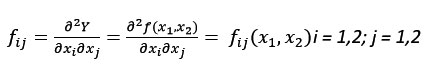
By distinguishing between the direct acceleration when i=j and cross acceleration when i≠j. When f_ij> 0, the marginal productivity f_i is increasing. When f_ij< 0 the marginal productivity f_i is decreasing. Further, if f_ij> 0 the two production factors are complementary (technically), i.e., an increase in the use of one of the input factors will increase the marginal productivity of the other input factor. If on the other hand fij< 0 the two input factors are substitutes, i.e., an increase in the use of one input factor reduces the marginal productivity of the other.   If f_ij = 0 then the input factors are technically independent. If the producer keeps adding one more unit of input, output will increase but the increase will become smaller (diminishing marginal return).

The Cobb-Douglas Production function

This is the most common type of production function introduced in 1928 by Cobb and Douglas,⁴ is used to show how inputs in the process of production lead to output, and other issues aside from production. It has the following properties.⁵

The first derivative of the inputs to output gives the marginal products of the inputs

Homogeneous of degree (α + β)

Linear in logarithms.

The value of (α + β) is the degree of returns to scale.

A unitary elasticity of substitution.

The expansion path generated by the production function is linear and passes through the origin.

The production function satisfies Euler’s Theorem: the output is exhausted by the production factors when the factors are paid for their marginal product.

Decreasing marginal productivity

The 2-factor Cobb-Douglas production function is given by:

Where:

Q is the output, L  is labor input, K is capital input, and A is total factor of productivity.

The following derivation shows how to determine the degree of returns to scale. Suppose all inputs were increased by a factor of t:

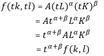
If α + β = 1, the function exhibits constant returns to scale.

Upon linearization using logarithms, the function becomes:

The constants a and β, respectively, are the elasticities of output to labour and capital inputs.

Modelling the economic output – Lessons from African Countries

Table 1: Summary table for comparison of supply models in three African countries

Key components of the models	Ethiopia	Malawi	Rwanda	Lesson for the Kenya model
Production function used	Not specified	Cobb-Douglas production function, and the Input-output model	Aggregate demand – aggregate supply side framework and CES function	Cobb-Douglas production function
Main sectors	Agriculture and non-agriculture sectors	Fiscal, monetary, real, and foreign sectors	Formal, informal, and agricultural sectors.	Agriculture, industry and services sectors
Number of behavioral or endogenous equations	14	Not specified	72	3
Main assumptions	Exogeneity of government expenditure and agricultural prices	Agriculture production for own use and for market; inputs from domestic and external markets.	The economy is supply-constrained	Aggregation of the 17 economic sectors into 3 broad sectors to compute Kenya’s GVA.

Ethiopia’s modelling of the agricultural output

The agriculture sector output for Ethiopia was done by Lemma.⁶ The agriculture sector is linked to the real relative price received by farmers, manufacturing supplies to the farming sector, and other exogenous variables related to weather and climate. The exogeneity of prices in the agriculture model has, however, been criticized by some studies, such that the exogeneity assumption will be unrealistic under external shocks such as war, drought, and terms of trade fluctuations.⁷

Rwanda’s estimation of the agriculture sector model

Rwanda’s supply-side economy is modelled into three key components: the formal, informal, and agricultural sectors. The production function is based on land, capital, technology, labour (mainly family labour), and rainfall to model supply from the agriculture sector. The agriculture sector is subdivided into cash crops and food production for the domestic market.⁸ The informal sector is defined to consist of small-scale industry and handicrafts, as well as informal trade activities such as street vendors and informal restaurant services. The formal sector consists mainly of the government and the modern private sectors of industry and services. Labour is determined by population growth.

Objectives, gaps, and Motivation for the Study

The study on modelling the agricultural sector gross value added is motivated by the need to understand the key drivers of total output in the agriculture sector, given that agriculture contributes about 18 per cent share to gross domestic product (GDP) and is a key sector in terms of employment generation in the rural areas and the mainstay for food security. This knowledge will be vital to policymakers in agriculture to identify relevant programs that will spur the growth of the agriculture sector and to put in place strategies aimed at boosting the productivity of the sector, both at the national and county levels.

The study fills a gap in the literature in the manner that there has been no study to date that has modelled the gross value added for Kenya’s agriculture sector, and especially from a macroeconomic perspective. The pioneer study will thus inspire additional studies in this sector including studies on productivity of the agriculture sector.

The overall objective of the study is thus to model the gross value added (GVA) of the agriculture sector of the Kenyan economy, and to generate projections for the GVA in the medium term. Specially, the study aimed to:

Identify the drivers of gross value added and model the GVA for Kenya’s agriculture sector,

Project the GVA for Kenya’s agriculture sector to the medium-term period, and

Propose policy options for raising production and boosting productivity in the agriculture sector.

Materials and Methods

Model specifications

The modeling of the agriculture sector is guided by three key African country-level papers^{6, 9-11} for Rwanda, Ethiopia, and Malawi, respectively.

The approach is through the Cobb-Douglas production function, in which output is modeled as a function of three key inputs, that is, capital, labour, and technology, presented as follows:

Where Y is total output, A is technology, K is capital, L is labor, and t represents time (annual).

Equation (1) can then be presented in the form of a cobb-Douglas production function as follows:

Where β and α represent the shares of capital and labor in production or total output, while (α+β) represents the returns to scale, so that if (α+β) =1 it means constant returns to scale, if (α+β)<1 it is decreasing returns to scale, and when (α+β)>1 it is increasing returns to scale.

The output from the various economic sectors is specified as a function of three key variables: capital stock (K), labor force (L), and technological progress (A). However, other control or exogenous variables explain the sectoral outputs, intermediate consumption, compensation of employees, sector expenditures, innovation index, environmental factors, among other sector-specific drivers such as enrolment in agricultural courses. Therefore, equation (2) is modified to allow for other control variables (Zt), as follows:

The summation of β, α, and δ provides the returns to scale of the production function. Before estimation, the assumption for the model restriction is as follows:

equation (4) implies that the production function assumes either constant or decreasing returns to scale.

Explanatory variables

The explanatory variables for the modelling have been deduced from both theoretical and empirical literature and utilizing variables available in the Kenyan context. Thus, table 2.1. below presents a summary of the variables for the sector’s estimated model. The variables are organized in a manner to reflect the Solow growth model where output is a function of capital stock, labour, technology, and other residual factors.

Table 2.1: Modelling economic output for the agriculture sector

Factors/ Sectors	Agriculture
Capital	·       Capital stock·       Total sector expenditure (absorption)·       Intermediate input (Fertilizer use)
Labor	·       Labor force·       Employee compensation
Technology	·       Enrolment in agricultural training courses
Other control variables	·       Environmental (land size, drought dummy)

Model specification for the agriculture gross value added

Total output in the agriculture sector is modelled as a function of 4 key variables: labour, capital, technology, and environmental factors. Hence, the model specification for agriculture output is as follows:

Where Agr-LF is the labour force in agriculture proxied by number of workers in the sector.  Assuming that labour is paid at marginal productivity, the model also incorporates compensation of employees as a proxy for the labour force. Cap-stock is capital stock (proxied by investment in the sector which is measured by gross fixed capital formation), other capital stock elements include intermediate inputs especially fertiliser use, and total expenditure in the agriculture sector which is proxied by total budget allocation. The Malabo declaration of 2014 requires that Governments allocate at least 10 percent of their budgets to agriculture. Env-factors are environmental factors (proxied by drought dummy and proportion of land size under agriculture), and Tech is technology (proxied by enrolment in agricultural training courses, which include Universities and Colleges). The global innovation index has also been captured as an additional control variable in the model. At the same time, βi are the model parameters to be estimated, and ε is the error term. The equations are expressed in logarithms to linearise the Cobb-Douglas production function. Gross value added is measured in Kenya shillings billions.

Variable types, measurement, and data sources

The variable types, measurements and sources of data are summarized in table 2.2 as shown. The factor inputs are obtained from the Cobb-Douglas production function with labour, capital, and technology as the key variables, and the last row representing other additional control variables for specific sectors.

Table 2.2: Variable types, measurement, and data sources

Factor inputs	Measurement of Variable	Unit of measure	Source of data
Labour (LF)	Compensation of employeesAgriculture labour force	Number in thousandsKsh million	KNBS Economic Surveys
Capital (Cap-stock)	·       Gross fixed capital formation (GFCF)·       Sector intermediate consumption·       Total sector expenditure by government	Ksh Billion	KNBS
Technology (Tech)	·       Enrolment in agricultural training courses in Universities and colleges.·       Fertilizer subsidy in Ksh billion·       Global Innovation Index (GII)	Number in thousandsKsh BillionIndex	KNBS
Control variables	Environmental factors Incidences of droughtProportion of total land size used for agriculture	Dummy variable where 1 is year there was drought, 0 is otherwiseThousand Sq Km	KNBSWorld Bank

Note: WIPO is the World Intellectual Property Organisation. *Fertilisers use proxies as intermediate agricultural inputs (in Ksh billion).

Data collection and cleaning

Data for the various variables were obtained from the Kenya National Bureau of Statistics using various Economic Surveys, Statistical Abstracts, and World Bank and WIPO databases. The data was collected from 1990 to 2023 annual time series data. The data was then cleaned for consistency by observing different base years.

Descriptive statistics

Table 3: Descriptive statistics for study variables

	AGRI_GVA	AGRI_LF	AGRIC_EXP in Ksh Billion	AGRIC_ LANDSIZE in 000’s Sq Km	CAP_ STOCK in Ksh Billion	ENROL_ ATI’s in Universities and colleges	FERT_ Subsidy in Ksh Billion	GII_ score (index)
Mean	661.90	319.05	29.00	272.12	958.78	9.83	7.76	27.51
Median	388.19	328	15.44	271.51	882.74	7.43	3.66	27.53
Max	1783.29	347	124.17	277.1	1897.01	25.458	30.11	31.85
Min	44.70	270	3.91	264.51	213.54	3.32	0.76	21.2
Std. Dev	603.67	22.97	27.32	4.20	544.25	6.31	8.03	2.47
J-B	4.59	4.96	21.00	2.59	2.88	5.32	13.01	0.72
Prob	0.1002	0.0836	0.0000	0.2731	0.2364	0.0698	0.0014	0.6943
Obs	34	34	34	34	34	34	34	34

NB: For the agriculture sector, total land size was used instead of as a proportion of total land since 80% of the landmass is ASAL. GFCF was the total but used across all three sectors.

Test for stationarity

Tests for unit roots include Phillips-Perron (PP), Augmented Dickey-Fuller (ADF), and Kwiatkowski-Phillips-Schmidt-Shin (KPSS).

Table 4: Unit root test using Augmented Dickey-Fuller Test

Variable	Unit root in levels t-statistic (p-value)	Unit root at 1st difference t-statistic (p-value)	Order of integration
Agric-gva	-1.7794 (0.6911)	-6.0608 (0.0001)	I (1)
Agric-lf	-1.9001 (0.6311)	-4.7751 (0.0044)	I (1)
Agric-exp	-1.3570 (0.8514)	-5.2246 (0.0011)	I (1)
Agric-landsize	-2.1000(0.5257)	-7.5005 (0.0000)	I (1)
Cs-gfcf	-1.9947 (0.5820)	-5.2606 (0.0009)	I (1)
Fert_use	3.2578 (1.0000)	-4.9208 (0.0026)	I (1)

Note: I (1) means stationary at first difference.

From the table, the variables used in the analysis are integrated in the first order.

Results

Estimation of the Agriculture Sector Output

Total output in the agriculture sector is modelled as a function of 7 variables: lagged agriculture GVA, labour force in agriculture, capital stock, climate change (proxied by drought), and resource allocation (total expenditure in agriculture). Lagged dependent variables are used to ensure modelling is dynamic rather than static and also based on the understanding that time series data assumes memory or inertia effects. The estimation is based on data for the period 1991 to 2023. The estimation for equation (6) is presented as follows:

Table 5: Agriculture sector estimation by Fully Modified Least Squares

Dependent Variable: LOG(AGRI_GVA)
Sample (adjusted): 1993 2023
Variable	Coefficient	Std. Error	t-Statistic	Prob.
LOG(AGRIC_EXP)	0.2102	0.0654	3.2127	0.0040
LOG(CAPITAL_STOCK_GFCF)	-0.2040	0.1266	-1.6116	0.1213
DROUGHT_1_(-2)	-0.0875	0.0313	-2.7940	0.0106
LOG(ENROLMENT_ATIs)	0.0612	0.0948	0.6462	0.5248
LOG(GII_KENYA_SCORE)	0.4916	0.1873	2.6243	0.0155
LOG(AGRI_GVA(-1))	0.6055	0.0965	6.2745	0.0000
LOG(EMPLOYEE_COMP_AGRIC)	0.1867	0.0896	2.0844	0.0489
LOG(FERTILIZER_USE)	0.0367	0.0936	0.3921	0.6987
C	-0.6098	0.7256	-0.8403	0.4098
R-squared	0.9848	Mean dep var		6.1707
Adjusted R-squared	0.9793	S.D. dep var		0.9833
S.E. of regression	0.1416	Sum sq resid		0.4409
Long-run variance	0.0054

Source: Estimation output based on study data. Prob is the probability value, t-stat is the t statistic.

The justification for using the FMOLS technique was that it is a useful method for estimating a long-term cointegrating relationship on the drivers of the agriculture sector. The relevant diagnostic tests were conducted, and the model was found to be suitable for use in the analysis and discussion of the model results, as presented in the next chapter.

Forecasting the agriculture sector total output

The estimated equation was then used to forecast the future values of the endogenous variables, that is, agriculture GVA.

Forecasts for the agriculture sector’s gross value added based on the estimated model

Table 6: Agriculture GVA Projections to medium term, 2025-2028.

Sector	2019	2020	2021	2022	2023	2024	2025	2026	2027	2028
Agric-GVA	1,631	1,706	1,700	1,675	1,783	1,906	1,959	2,120	2,217	2,322
Agricshare	19%	20%	18%	17%	17%	17%	17%	17%	17%	17%

Source: Estimated projections from the FMOLS equation

Discussion

Discussion of results

The study aimed at modelling the total output in the agriculture sector as measured by gross value added, and to forecast the sector’s GVA to the medium term. This was achieved by using the Cobb-Douglas production function approach and analyzing the data using the fully modified OLS cointegration technique. The explanatory variables used model in the analysis were labour force in agriculture, capital stock, climate change (proxied by drought), resource allocation (total expenditure in agriculture), and the lagged agriculture GVA. The estimation for the agriculture sector GVA is based on data for the period 1991 to 2023.

Based on the study model, expenditure in the agriculture sector had a positive and significant elasticity of 0.21. Every one percent increase in expenditure to the sector would therefore translate to a 0.21 percent increase in gross value added (GVA) to the sector. This finding therefore reiterates the need to observe the 2014 Malabo Declaration that called for at least 10 to 15 per cent of the national expenditure to be directed to the agriculture sector. On the other hand, drought harmed GVA in the agriculture sector with an estimated elasticity of -0.09, which emphasizes that drought or unfavorable weather conditions negatively affect agricultural output. This means that investment in irrigation and moving away from rainfed agriculture would be a worthwhile investment to pursue for stable production by the sector. Capital stock was found to be insignificant, and this was due to the lack of data for capital stock in the sector, thus, the study proxied capital stock by the entire gross fixed capital formation (GFCF) in the overall economy.

Technology and innovation were also found to be significant in affecting output in the sector, with a 0.49 degree of elasticity. Technology and innovation were proxied by the Global Innovation Index (GII) score and enrolment in agricultural training institutions (ATIs). Enrolment in ATIs also yielded a positive elasticity as expected, of 0.06, but the coefficient t was, however, not significant. Thus, the adoption of technologies and innovations in the sector is likely to lead to higher output or production in the agriculture sector. On the other hand, compensation of employees in the sector had a significant elasticity of 0.18, as expected. Employee compensation was used to capture returns to farmers from their labour and how that is likely to motivate them to continue engaging in farming. This result implies that measures that ensure farmers get good returns from their hard work should be put in place, since experience has shown that farmers do not get the full value of their produce, especially in markets where middlemen exploit them. The agricultural value chain should thus ensure that value is created at each stage, and the farmer gets their rightful share of the value.

The persistence or inertia effects of lagged GVA in the sector were 0.60, which means that the previous sector GVA had a 0.60 share in determining the GVA for the net period, on average. While fertilizer use is key for agricultural production, there has been limited data on fertilizer use, hence the insignificance of the estimated coefficient, and on account that Kenya embarked on a fertilizer subsidy in recent years. This, therefore, forms a potential area for future research work to understand how the subsidy and the use of fertilizer affect agricultural production.

Forecasting the agriculture sector total output

The estimated equation was then used to forecast the future values of the endogenous variables, that is, agriculture GVA.

Based on the FMOLS cointegration equation, the GVA for the agriculture sector is expected to increase from Ksh 1,783 million in 2023 to Ksh 2,322 million in 2028. The estimated projections will thus contribute to the country’s overall GDP since the share of agriculture in GDP is about 17 per cent. These projections make an assumption that there will be continued expenditure by the government to the sector, there will be continuous innovation and technology adoption, no extreme weather events such as droughts or floods, and that measures to ensure farmers are effectively compensated for their production will be put in place; as well as other programmes by the Government to enhance the productivity of the sector, which is crucial for food security, job creation, and economic growth.

Conclusion and Policy Implications

The study gives cognizance to the importance of the Cobb-Douglas production functions. An estimation was undertaken for the Gross Value Added for the Agriculture sector and then used to project the future values of GVA in the sector. The projection for the agriculture sector from the model was from Ksh 1.78 trillion in 2023 to an estimated Ksh 2.32 trillion in 2028.

The policy implications for the study are thus summarized as follows:

Targeted subsidies of production inputs to support agricultural production, especially fertilizer, seeds, and other inputs

Invest in irrigated agriculture since relying on rain-fed agriculture poses a risk to food security.

Despite fiscal constraints, observe the Malabo Declaration of ensuring 10-15 per cent of national expenditure on the agriculture sector.

Focus on developing agricultural value chains to ensure that the sector creates income and employment opportunities, such as through the export of agricultural commodities. Ensuring also that farmers get well compensated for their hard work within the value chain, and to overcome instances of farmer exploitation.

Value addition through agro-processing firms at the national and county levels, to raise productivity in the agricultural sector.

Acknowledgement

The author(s) would like to thank other researchers from KIPPRA who offered technical support in developing the article. These include Dr. Rose Ngugi, Former Executive Director at KIPPRA; Dr. Eldah Onsomu, Ag. Executive Director at KIPPRA; Mr. Benson Kiriga, State Department for Economic Planning; Dr. James Ochieng, UNICEF; Ms. Hellen Chemnyongoi, UNICEF; Mr. Daniel Omanyo, and a host of other KIPPRA Colleagues. Much appreciation to Former Colleagues and Students at Kenyatta University, School of Economics. The author is also profoundly grateful to the many reviewers who gave comments in the initial stages, including Cyrus Mutuku (KRA), Dr. Tom Mukhongo (Laikipia University), Dr. James Murunga (Machakos University), Dr. Owen Nyangoro (University of Nairobi), Dr. Maureen Were (CBK), and Mr. Noah Wasike (Institute of Economic Affairs). We also thank the Current Agriculture Research Journal and the editors and reviewers for seeing through this manuscript.

Funding Sources

The author(s) received no financial support for the research, authorship, and/or publication of this article.

Conflict of Interest

The author does not have any conflict of interest.

Data availability statement

The manuscript incorporates all datasets produced or examined throughout this research study.

Informed Consent Statement

This study did not involve an experiment on humans and animals, and therefore, informed consent was not required.

Ethics statement

This research did not involve human participants, animal subjects, or any material that requires ethical approval.

Permission to reproduce material from other sources

Not applicable.

Author Contributions

The sole author was responsible for the conceptualization, methodology, data collection, analysis, writing, and final approval of the manuscript.

References

1. Hicks, John R. “Marginal productivity and the principle of variation.” Economica 35 (1932): 79-88.
   CrossRef
2. Harrod, R. F. “Value and capital.” The Economic Journal 49.194 (1939): 294-300.
   CrossRef
3. Solow, Robert M. “A contribution to the theory of economic growth.” The quarterly journal of economics 70.1 (1956): 65-94.
   CrossRef
4. Cobb, Charles W., and Paul H. Douglas. “A theory of production.” The American economic review1 (1928): 139-165.
5. Geda, Alemayehu, and Addis Yimer. “An applied dynamic structural macro-econometric model for Rwanda.” Studies in Economics and Econometrics 46.4 (2022): 249-281.
   CrossRef
6. Geda, Alemayehu, and Daniel Zerfu. “A Review of Macro Modelling in Ethiopia.” (2004).
7. Geda, Alemayehu, and Addis Yimer. “An applied macro-econometric model for supply constrained African economy: A Rwandan macro model.” Tanzanian Economic Review1-2 (2014).
   CrossRef
8. Gurara, Daniel Zerfu. A macroeconometric model for Rwanda. African Development Bank Group, 2013.
9. Lemma, M. ‘Modelling the Ethiopian Economy: Experience and Prospects’. 1993. (memo).
10. Mandal, Ram Krishna. Microeconomic theory. Atlantic Publishers & Dist, 2007.
11. Choudhury, Robin. “Macroeconomic modelling in developing countries.” Statistics Norway, Reports(2012).

Abbreviations List

AGR                 Agriculture sector

CAP                 Capital stock

CES                  Constant Elasticity of Substitution

FMOLS             Fully Modified Ordinary Least Squares method

GDP                 Gross Domestic Product

GVA                 Gross Value Added

MRTS               Marginal Rate of Technical Substitution

SAP                  Structural Adjustment Programme

TECH               Technology

WIPO               World Intellectual Property Organization

Appendix

Table A.1: Re-estimation of agriculture sector equation for a static equation

Dependent Variable: LOG(AGRI_GVA)
Method: Fully Modified Least Squares (FMOLS)
Sample (adjusted): 1993 2023
Variable	Coefficient	Std. Er	t-Stat	Prob.
LOG(AGRIC_EXP)	0.1962	0.1416	1.3858	0.1791
LOG(CAP_STOCK_GFCF)	-0.0074	0.2386	-0.0310	0.9755
DROUGHT_1_(-2)	-0.0109	0.0546	-0.2002	0.8431
LOG(ENROL_ATI_S__000_S_)	0.0845	0.1789	0.4721	0.6413
LOG(FERTILIZER_USE(-1))	0.3861	0.2060	1.8741	0.0737
LOG(GII_KENYA_SCORE)	0.6364	0.3527	1.8045	0.0843
LOG(EMPLOYEE_COMP_AGRIC_KSHM_)	0.3092	0.1909	1.6200	0.1189
C	-0.6796	1.4604	-0.4654	0.6460
R-squared	0.9777	Mean dependent var		6.1707
Adjusted R-squared	0.9709	S.D. dependent var		0.9833
Long-run variance	0.0194

Source: EViews estimation based on source data.